In this post, we are gonna briefly go over the field of Reinforcement Learning (RL), from fundamental concepts to classic algorithms. Hopefully, this review is helpful enough so that newbies would not get lost in specialized terms and jargons while starting. [WARNING] This is a long read.
- Why transfer learning?
- What is transfer learning
- Different scenarios in transfer learning
- Ways to use transfer learning
- Working through an example
If we think intuitively, it is not realistic and practical for us to learn everything from scratch. We always try to solve a new task based on the knowledge obtained from past experiences. For example, we may find that learning to recognize apples might help to identify pears, or learning a programming language, say C++, can facilitate learning some other language, say Python, as the basic programming fundamentals remain the same.
Transfer learning is an area of deep learning inspired by the same idea. We try to use the “knowledge” acquired in one task to do some other related task. This is mainly motivated by the lack of labeled data across domains. A simple example would be the ImageNet dataset, which has millions of images of different categories. However, getting such a dataset for every domain is challenging. Besides, most deep learning models are very specialized to a particular domain or even a specific task. They have high accuracy and beat all benchmarks, but only on particular datasets, and end up suffering a significant loss in performance when used in a new task that might still be similar to the one it was trained on.
Why transfer learning?
 |
 |
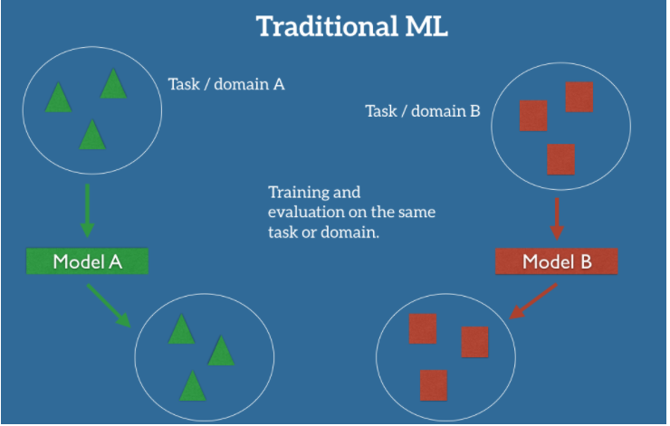
In the classic supervised learning scenario of machine learning, we use labeled data to train a model on a specific task and domain $A$. Say, we are considering the problem of sentiment classification, where the task is to automatically classify the reviews on a product, such as a brand of camera, into positive and negative views. Now the distribution of review data for different types of products can be dissimilar, so to maintain good classification performance on all the products, we need to collect a large amount of labeled data for every product.
However, this kind of data labeling is very expensive to do. To reduce this effort, we may want to train a few classification networks and then adapt the learning for some other products. This is where transfer learning kicks in. We are essentially trying to use some trained network to make predictions on a related task that is different from what the network was initially trained on.
What is transfer learning
To go further, we need to familiarize ourselves with some notations and definitions.
-
Domain : Given a specific dataset $X = \set{x_1, … , x_n} ∈ X$ , where $X$ denotes the feature space, and a marginal probability distribution on the dataset $P(X)$. A domain can be defined as $D(X, P(X))$. For example, if our learning task is document classification, and each word is taken as a binary feature, then $X$ is the space of all word vectors, $x_i$ is the $i$th word vector corresponding to some documents, and $X$ is a particular learning sample. In general, if two domains are different, then they may have different feature spaces or different marginal probability distributions.
-
Task : For a specific domain, $D = {X, P(X)}$, a task consists of two components: a label space $Y$ and an predictive function $f(·)$ (denoted by $T = {Y, f(·)}$), which is learned from the training data, which consist of pairs $ \set{x_i, y_i}$, where $x_i ∈ X$ and $y_i ∈ Y$. The predictive function $f(.)$ can be seen as a conditional distribution $P(Y|X)$. In our document classification example, Y is the set of all labels, which is True, False for a binary classification task.
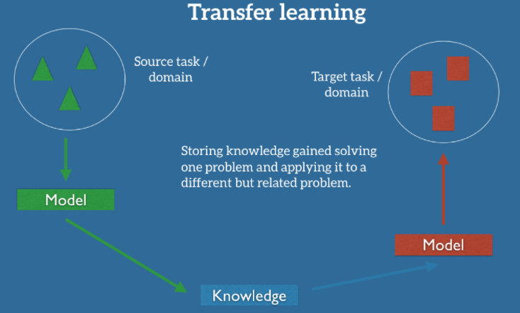
Now that we understand what a domain and a task is, we take the formal definition of transfer learning from a paper written by Pan and Yang1
Transfer Learning: Given a source domain $D_s$ and its corresponding task $T_s$, where the learned function $f_s$ can be interpreted as some knowledge obtained in $D_s$ and $T_s$. Our goal is to get the target predictive function $f_t$ for target task $T_t$ with target domain $D_t$. Transfer learning aims to help improve the performance of $f_t$ by utilizing the knowledge $f_s$, where $D_s \neq D_t$ or $T_s \neq T_t$. In short, transfer learning can be simply denoted as $\begin{align} D_s, T_s \rightarrow D_t, T_t \end{align}$
Different scenarios in transfer learning
Based on $D_s \neq D_t$ or $T_s \neq T_t$. , we can have three scenarios when applying transfer learning.
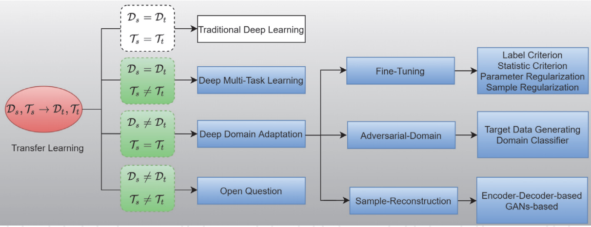
When $D_s = D_t$ and $T_s = T_t$, the problem becomes a traditional deep learning task. In such case, a dataset is usually divided into a training dataset $D_s$ and a test training dataset $D_t$, then we can train a neural network $F$ on $D_s$ and apply the pre-trained model $F$ to $D$
When the domains are the same, i.e., $D_s$ = $D_t$ and $T_s \neq T_t$, the problem becomes a multi-task learning problem i.e., As the source domain and the target domain has the same feature space, we can utilize one giant neural network to solve different types of tasks simultaneously. If the tasks are different, then either
- The label spaces between the domains are different, i.e. $Y_s \neq Y_t$ or
- The conditional probability distributions between the domains are different; i.e. $P(Y_s|X_s) \neq P(Y_t|X_t)$
In our document classification example, case 1 corresponds to the situation where the source domain has binary document classes, whereas the target domain has ten classes to classify the documents. Case 2 corresponds to the situation where the source and target documents are very unbalanced in terms of the user-defined classes.
Finally, If the domains are different and $T_s$ is similar to $T_t$, we use deep domain adaptation techniques. Where the goal of domain adaptation is to learn $f_t$ from $f_s$ when we change domains. Clearly when $D_s \neq D_t$ either
- The feature spaces between the domains are different, i.e. $X_s \neq X_t$ , or
- The feature spaces between the domains are the same, but the marginal probability distributions between domain data are different i.e., $P(X_s) \neq P(X_t)$
For example, in our document classification example, case 1 corresponds to when the two sets of documents are described in different languages. Case 2 may correspond to when the source domain documents and the target domain documents focus on different topics.
As a side note, when $D_s \neq D_t$ and $T_s \neq T_t$, transfer learning becomes complicated. Sometimes transferring knowledge from some other model may lead to worse performance. This is technically called negative learning. Suppose the data in the source domain $D_s$ is very different from that in target domain $D_t$. In that case, brute force transfer may hurt the performance of predictive function $F_t$, not to mention the scenario when source task $T_s$ and target task $T_t$ are also different. This is still an area of open research. You can read this survey paper
Ways to use transfer learning
Now that we understand transfer learning, we are faced with the question of how to apply transfer learning. The essential idea is to use a pre-trained network and then tweak it to serve our purpose. Coming from traditional machine learning, if we wanted to use our network, we will load it in memory and give it an example to make predictions on. The network then feed forwards this example to all the layers and gives us the prediction. Usually, in deep neural networks, just before the output, a fully connected layer utilizes whatever the network has learned into making its final prediction. So if we were to use this network’s “knowledge,” we have several options to extract it.
For simplicity’s sake, let’s take the example of a ConvNet trained on the ImageNet dataset (Alexnet, for example) and understand how we can use this to transfer the knowledge.
 Vanilla CNN ; CNN as a feature extractor ; CNN with fine tuning and feature extraction
-
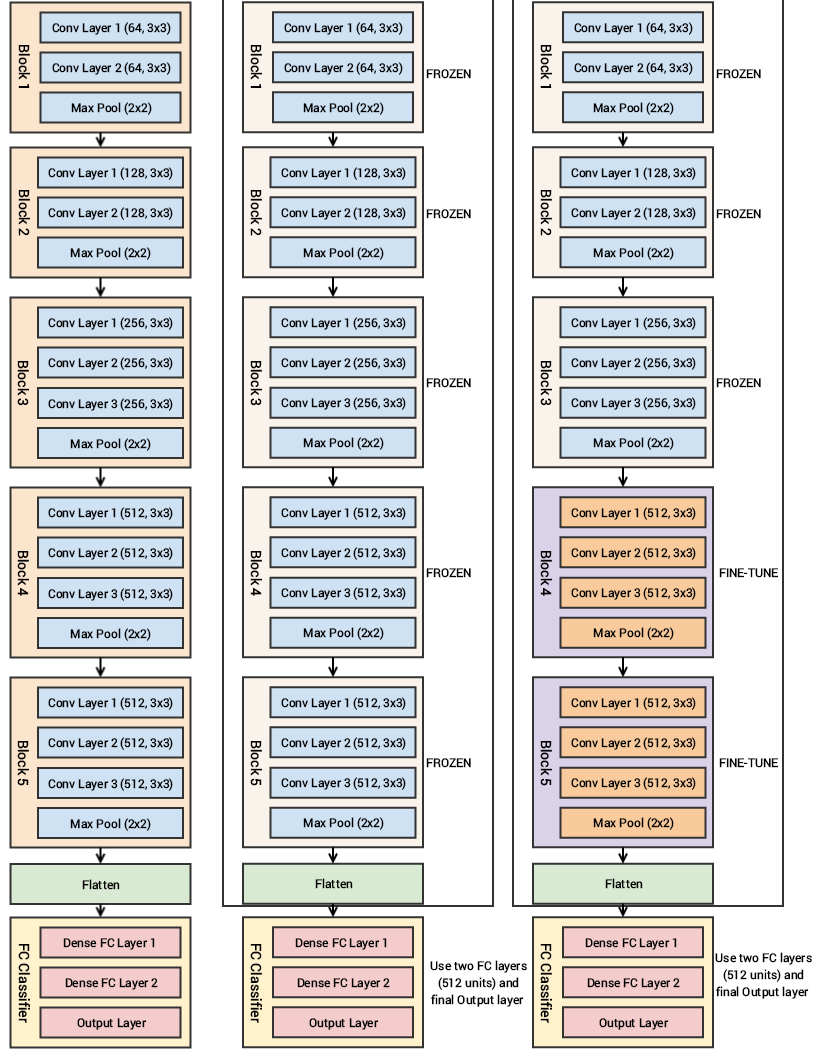
As a fixed feature extractor: Here, the idea is to take a ConvNet pre-trained on ImageNet, remove the last fully-connected layer (the layer having its outputs as the 1000 class scores for a different task), then treat the rest of the ConvNet as a fixed feature extractor for the new dataset. In essence, we are only using this network to get the final feature map of the input. In an AlexNet, this would compute a 4096-D vector for every image that contains the activations of the hidden layer immediately before the classifier. We call these features CNN codes. It is essential for performance that these codes are ReLUd (yeah, that’s a word) i.e., thresholded at zero if they were also thresholded during the training of the ConvNet(as is usually the case). Once we extract the 4096-D codes for all images, train a linear classifier (e.g. Linear SVM or Softmax classifier) for the new dataset.
-
Fine-tuning the ConvNet: It will not always be sufficient for us to just use the network as it is and make do with letting go of the final layer. So, the second strategy is to not only replace and retrain the classifier on top of the ConvNet on the new dataset but to also fine-tune the weights of the pre-trained network by continuing the backpropagation. It is possible to fine-tune all the layers of the ConvNet, or it is possible to keep some of the earlier layers fixed (due to overfitting concerns) and only fine-tune some higher-level portion of the network. This is motivated by the observation that the earlier features of a ConvNet contain more generic features (e.g. edge detectors or color blob detectors) that should be useful to many tasks. However, later layers of the ConvNet become progressively more specific to the details of the classes contained in the original dataset. In the case of ImageNet, which contains many dog breeds, a significant portion of the representational power of the ConvNet may be devoted to features that are specific to differentiating between dog breeds.
-
Pretrained models. Since modern ConvNets take 2-3 weeks to train across multiple GPUs on ImageNet, it is common to see people release their final ConvNet checkpoints to benefit others who can use the networks for fine-tuning. For example, the Caffe library has a Model Zoo where people share their network weights.
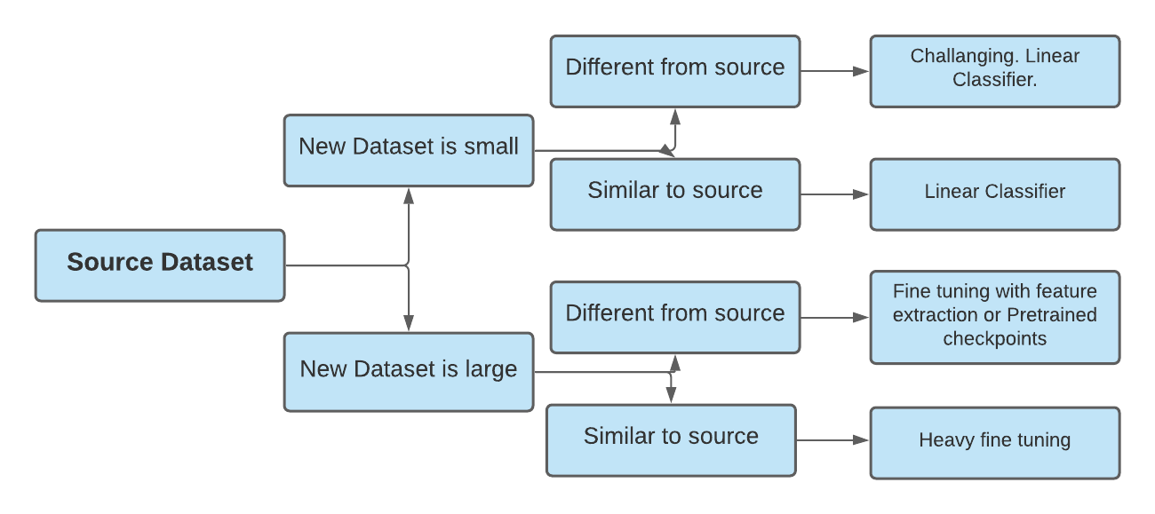
Now that we know how domain and task can differ and how we intend to use the pre-trained network, here are some ideas so as to how to use transfer learning in a given context.
-
New dataset is small and similar to the original dataset: Training neural networks on small datasets can lead to overfitting, so fine-tuning the network is not a good idea. However, since the datasets are similar higher-level features in the ConvNet will be relevant. So training a linear classifier on CNN nodes is a good idea in this case.
-
New dataset is large and similar to the original dataset: This is the best-case scenario. Since we have a lot of data, we can fine-tune the network with ease without worrying about overfitting. The best idea, hence, is to fine-tune the network
-
New dataset is small but very different from the original dataset: This is a challenging problem of domain adaptation. As explained earlier, since the data is small, it is likely best to only train a linear classifier. Since the dataset is very different, it might not be best to train the classifier from the top of the network, which contains more dataset-specific features. Instead, it might work better to train the SVM classifier from activations somewhere earlier in the network. Using a prior checkpoint in the pre-trained network will work best in this case. However, there are chances of negative transfer.
-
New dataset is large and very different from the original dataset: Since the dataset is very large, we may expect that we can afford to train a ConvNet from scratch. However, in practice, it is very often still beneficial to initialize with weights from a pre-trained model. In this case, we would have enough data and confidence to fine-tune through the entire network.
Working through an example
As with everything, it’s good to practice a few problems when you learn a new technique. I found this classic dog and cat classification problem on Kaggle that was recommended in a blog post.
In this challange we are to write an algorithm to classify whether images contain either a dog or a cat. The problem gives us a dataset containing 25,000 labeled images. We can of course write a CNN from scratch and use it for prediction, but that will take considerably more effort and time than if we were to ‘transfer’ the knowledge required to classify images from some another model. We’ll use VGG-19 as our pretrained model in this case.
I figure out that my setup is a kind of case when it’s recommended to use a pretrained model and frezze the parameters (different domain, same task, small dataset) while only using the last layer.
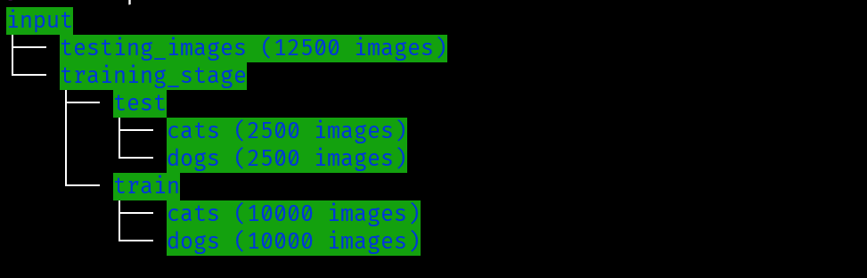
So starting off we’ll write a custom dataset and use Dataloader to load our data which i’ve divided in this format
class custom_data_loader(Dataset):

  def __len__(self):
    return len(self.file_list)

  def __getitem__(self, idx):
     img = Image.open(os.path.join(self.dir, self.file_list[idx]))
     if self.transform:
      img = self.transform(img)
     if self.mode == 'train':
      img = img.numpy()
      return img.astype('float32'), self.label
     else:
      img = img.numpy()
      return img.astype('float32'), self.file_list[idx]
# number of subprocesses to use for data loading
num_workers = 0
# how many samples per batch to load
batch_size = 32

test_dir = 'input_data/test1'
test_files = os.listdir(test_dir)

# convert data to a normalized torch.FloatTensor
train_transforms = transforms.Compose([transforms.Resize((224,224)),
                                      transforms.ToTensor(),
                                      transforms.Normalize([0.485, 0.456, 0.406],
                                                           [0.229, 0.224, 0.225])])

valid_transforms = transforms.Compose([transforms.Resize((224,224)),
                                      transforms.ToTensor(),
                                      transforms.Normalize([0.485, 0.456, 0.406],
                                                           [0.229, 0.224, 0.225])])
# choose the training and test datasets

test_transforms = transforms.Compose([transforms.Resize((224,224)),
                                      transforms.ToTensor(),
                                      transforms.Normalize([0.485, 0.456, 0.406],
                                                           [0.229, 0.224, 0.225])])
# choose the training and test datasets
train_data = datasets.ImageFolder('input_data/training_stage/train', transform=train_transforms)
valid_data=datasets.ImageFolder('input_data/training_stage/test',transform=valid_transforms)
test_data = custom_data_loader(test_files, test_dir, transform=test_transforms)
# prepare data loaders (combine dataset and sampler)
train_loader = torch.utils.data.DataLoader(train_data, batch_size=batch_size, num_workers=num_workers,shuffle=True)
valid_loader = torch.utils.data.DataLoader(valid_data, batch_size=batch_size,  num_workers=num_workers,shuffle=True)
test_loader = torch.utils.data.DataLoader(test_data, batch_size=batch_size,  num_workers=num_workers)
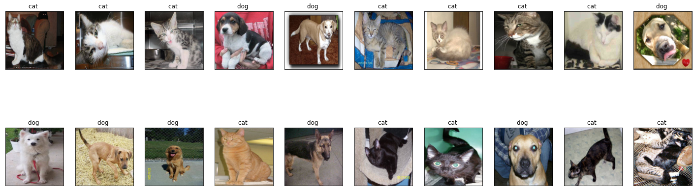
Training images given to us are of this type.
# Get some training images
dataiter = iter(train_loader)
images, labels = dataiter.next()

# plot the images in the batch, along with the corresponding labels
fig = plt.figure(figsize=(25, 8))

# display some images along with labels
for idx in np.arange(20):
    ax = fig.add_subplot(2, 20/2, idx+1, xticks=[], yticks=[])
    imshow(images[idx])
    ax.set_title("{} ".format( classes[labels[idx]]))
Now comes the transfer learning part. We’ll load VGG-19 into memory and then frezze the layers and examine the model. We’ll also set our criterion, optimizer and scheduler.
vgg_19=models.vgg19_bn(pretrained=True)
vgg_19
Downloading: "https://download.pytorch.org/models/vgg19_bn-c79401a0.pth" to /root/.cache/torch/hub/checkpoints/vgg19_bn-c79401a0.pth
# Freeze parameters so we don't backprop through them
for param in vgg_19.parameters():
    param.requires_grad = False

from collections import OrderedDict
classifier = nn.Sequential(OrderedDict([
                          ('fc1', nn.Linear(25088, 1028)),
                          ('relu1', nn.ReLU()),
                          ('dropout1',nn.Dropout(0.5)),
                          ('fc2', nn.Linear(1028, 512)),
                          ('relu2', nn.ReLU()),
                          ('dropout2',nn.Dropout(0.5)),
                          ('fc3', nn.Linear(512, 2)),
                          ('output', nn.LogSoftmax(dim=1))
                          ]))

vgg_19.classifier = classifier
# Model
vgg_19

# Criteria NLLLoss which is recommended with Softmax final layer
criterion = nn.NLLLoss()

# Observe that all parameters are being optimized
optimizer = torch.optim.Adam(vgg_19.classifier.parameters(), lr=0.001)

# Decay LR by a factor of 0.1 every 3 epochs
scheduler = lr_scheduler.StepLR(optimizer, step_size=3, gamma=0.1)
VGG(
  (features): Sequential(
    (0): Conv2d(3, 64, kernel_size=(3, 3), stride=(1, 1), padding=(1, 1))
    (1): BatchNorm2d(64, eps=1e-05, momentum=0.1, affine=True, track_running_stats=True)
    (2): ReLU(inplace=True)
    (3): Conv2d(64, 64, kernel_size=(3, 3), stride=(1, 1), padding=(1, 1))
    (4): BatchNorm2d(64, eps=1e-05, momentum=0.1, affine=True, track_running_stats=True)
    (5): ReLU(inplace=True)
    (6): MaxPool2d(kernel_size=2, stride=2, padding=0, dilation=1, ceil_mode=False)
    (7): Conv2d(64, 128, kernel_size=(3, 3), stride=(1, 1), padding=(1, 1))
    (8): BatchNorm2d(128, eps=1e-05, momentum=0.1, affine=True, track_running_stats=True)
    (9): ReLU(inplace=True)
    (10): Conv2d(128, 128, kernel_size=(3, 3), stride=(1, 1), padding=(1, 1))
    (11): BatchNorm2d(128, eps=1e-05, momentum=0.1, affine=True, track_running_stats=True)
    (12): ReLU(inplace=True)
    (13): MaxPool2d(kernel_size=2, stride=2, padding=0, dilation=1, ceil_mode=False)
    (14): Conv2d(128, 256, kernel_size=(3, 3), stride=(1, 1), padding=(1, 1))
    (15): BatchNorm2d(256, eps=1e-05, momentum=0.1, affine=True, track_running_stats=True)
    (16): ReLU(inplace=True)
    (17): Conv2d(256, 256, kernel_size=(3, 3), stride=(1, 1), padding=(1, 1))
    (18): BatchNorm2d(256, eps=1e-05, momentum=0.1, affine=True, track_running_stats=True)
    (19): ReLU(inplace=True)
    (20): Conv2d(256, 256, kernel_size=(3, 3), stride=(1, 1), padding=(1, 1))
    (21): BatchNorm2d(256, eps=1e-05, momentum=0.1, affine=True, track_running_stats=True)
    (22): ReLU(inplace=True)
    (23): Conv2d(256, 256, kernel_size=(3, 3), stride=(1, 1), padding=(1, 1))
    (24): BatchNorm2d(256, eps=1e-05, momentum=0.1, affine=True, track_running_stats=True)
    (25): ReLU(inplace=True)
    (26): MaxPool2d(kernel_size=2, stride=2, padding=0, dilation=1, ceil_mode=False)
    (27): Conv2d(256, 512, kernel_size=(3, 3), stride=(1, 1), padding=(1, 1))
    (28): BatchNorm2d(512, eps=1e-05, momentum=0.1, affine=True, track_running_stats=True)
    (29): ReLU(inplace=True)
    (30): Conv2d(512, 512, kernel_size=(3, 3), stride=(1, 1), padding=(1, 1))
    (31): BatchNorm2d(512, eps=1e-05, momentum=0.1, affine=True, track_running_stats=True)
    (32): ReLU(inplace=True)
    (33): Conv2d(512, 512, kernel_size=(3, 3), stride=(1, 1), padding=(1, 1))
    (34): BatchNorm2d(512, eps=1e-05, momentum=0.1, affine=True, track_running_stats=True)
    (35): ReLU(inplace=True)
    (36): Conv2d(512, 512, kernel_size=(3, 3), stride=(1, 1), padding=(1, 1))
    (37): BatchNorm2d(512, eps=1e-05, momentum=0.1, affine=True, track_running_stats=True)
    (38): ReLU(inplace=True)
    (39): MaxPool2d(kernel_size=2, stride=2, padding=0, dilation=1, ceil_mode=False)
    (40): Conv2d(512, 512, kernel_size=(3, 3), stride=(1, 1), padding=(1, 1))
    (41): BatchNorm2d(512, eps=1e-05, momentum=0.1, affine=True, track_running_stats=True)
    (42): ReLU(inplace=True)
    (43): Conv2d(512, 512, kernel_size=(3, 3), stride=(1, 1), padding=(1, 1))
    (44): BatchNorm2d(512, eps=1e-05, momentum=0.1, affine=True, track_running_stats=True)
    (45): ReLU(inplace=True)
    (46): Conv2d(512, 512, kernel_size=(3, 3), stride=(1, 1), padding=(1, 1))
    (47): BatchNorm2d(512, eps=1e-05, momentum=0.1, affine=True, track_running_stats=True)
    (48): ReLU(inplace=True)
    (49): Conv2d(512, 512, kernel_size=(3, 3), stride=(1, 1), padding=(1, 1))
    (50): BatchNorm2d(512, eps=1e-05, momentum=0.1, affine=True, track_running_stats=True)
    (51): ReLU(inplace=True)
    (52): MaxPool2d(kernel_size=2, stride=2, padding=0, dilation=1, ceil_mode=False)
  )
  (avgpool): AdaptiveAvgPool2d(output_size=(7, 7))
  (classifier): Sequential(
    (fc1): Linear(in_features=25088, out_features=1028, bias=True)
    (relu1): ReLU()
    (dropout1): Dropout(p=0.5, inplace=False)
    (fc2): Linear(in_features=1028, out_features=512, bias=True)
    (relu2): ReLU()
    (dropout2): Dropout(p=0.5, inplace=False)
    (fc3): Linear(in_features=512, out_features=2, bias=True)
    (output): LogSoftmax(dim=1)
  )
)
Now we’ll train our model.
# training on GPU
vgg_19.cuda()

# number of epochs to train the model
n_epochs = 9

# Initilize the validation loss to infinity
valid_loss_min = np.Inf

for epoch in range(1, n_epochs+1):

    # Initialize training and validation loss
    train_loss = 0.0
    valid_loss = 0.0

    # Re-training parts of this model
    vgg_19.train()

    for data, target in train_loader:

        # move tensors to GPU
        data, target = data.cuda(), target.cuda()

        # clear the gradients of all optimized variables
        optimizer.zero_grad()

        # forward pass: compute predicted outputs by passing inputs to the model
        output = vgg_19(data)

        # calculate the batch loss
        loss = criterion(output, target)

        # backward pass: compute gradient of the loss with respect to model parameters
        loss.backward()

        # perform a single optimization step (parameter update)
        optimizer.step()

        # update training loss
        train_loss += loss.item()*data.size(0)

    # Validating the model
    vgg_19.eval()

    for data, target in valid_loader:

        # move tensors to GPU
        data, target = data.cuda(), target.cuda()

        # forward pass: compute predicted outputs by passing inputs to the model
        output = vgg_19(data)

        # calculate the batch loss
        loss = criterion(output, target)

        # update average validation loss
        valid_loss += loss.item()*data.size(0)


    train_loss = train_loss/len(train_loader.dataset)
    valid_loss = valid_loss/len(valid_loader.dataset)

    # print training/validation statistics
    print('Epoch: {} \tTraining Loss: {:.6f} \tValidation Loss: {:.6f}'.format(
        epoch, train_loss, valid_loss))

    # save model if validation loss has decreased
    if valid_loss <= valid_loss_min:
        print('Validation loss decreased ({:.6f} --> {:.6f}).  Saving model ...'.format(
        valid_loss_min,
        valid_loss))
        torch.save(vgg_19.state_dict(), 'model_vgg19.pth')
        valid_loss_min = valid_loss
/usr/local/lib/python3.7/dist-packages/torch/nn/functional.py:718: UserWarning: Named tensors and all their associated APIs are an experimental feature and subject to change. Please do not use them for anything important until they are released as stable. (Triggered internally at  /pytorch/c10/core/TensorImpl.h:1156.)
  return torch.max_pool2d(input, kernel_size, stride, padding, dilation, ceil_mode)


Epoch: 1  Training Loss: 0.996212   Validation Loss: 0.105541
Validation loss decreased (inf --> 0.105541).  Saving model ...
Epoch: 2  Training Loss: 0.777823   Validation Loss: 0.145331
Epoch: 3  Training Loss: 1.044374   Validation Loss: 0.072210
Validation loss decreased (0.105541 --> 0.072210).  Saving model ...
Validating the model
batch_size=4

# track test loss
test_loss = 0.0
class_correct = list(0. for i in range(2))
class_total = list(0. for i in range(2))

vgg_19.eval()
# iterate over valid data
for data, target in valid_loader:
    # move tensors to GPU if CUDA is available
    if train_on_gpu:
        data, target = data.cuda(), target.cuda()
    # forward pass: compute predicted outputs by passing inputs to the model
    output = vgg_19(data)
    # calculate the batch loss
    loss = criterion(output, target)
    # update test loss
    test_loss += loss.item()*data.size(0)
    # convert output probabilities to predicted class
    _, pred = torch.max(output, 1)
    # compare predictions to true label
    correct_tensor = pred.eq(target.data.view_as(pred))
    correct = np.squeeze(correct_tensor.numpy()) if not train_on_gpu else np.squeeze(correct_tensor.cpu().numpy())
    # calculate test accuracy for each object class
    for i in range(batch_size):
        label = target.data[i]
        class_correct[label] += correct[i].item()
        class_total[label] += 1

# average test loss
test_loss = test_loss/len(valid_loader.dataset)
print('Test Loss: {:.6f}\n'.format(test_loss))

for i in range(2):
    if class_total[i] > 0:
        print('Test Accuracy of %5s: %2d%% (%2d/%2d)' % (
            classes[i], 100 * class_correct[i] / class_total[i],
            np.sum(class_correct[i]), np.sum(class_total[i])))
    else:
        print('Test Accuracy of %5s: N/A (no training examples)' % (classes[i]))

print('\nTest Accuracy (Overall): %2d%% (%2d/%2d)' % (
    100. * np.sum(class_correct) / np.sum(class_total),
    np.sum(class_correct), np.sum(class_total)))
Test Loss: 0.072210

Test Accuracy of   cat: 92% (171/184)
Test Accuracy of   dog: 100% (192/192)

Test Accuracy (Overall): 96% (363/376)
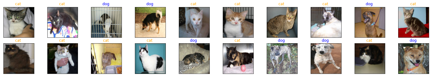
Let’s see how our model performs on the test dataset
batch_size=32

test_loader = torch.utils.data.DataLoader(test_data, batch_size=batch_size,  num_workers=num_workers)
vgg_19.cpu()

# obtain one batch of test images
dataiter = iter(test_loader)
images, labels = dataiter.next()

# get predictions
output = vgg_19(images)

# convert output probabilities to predicted class
_, preds_tensor = torch.max(output, 1)
preds = np.squeeze(preds_tensor.numpy()) if not train_on_gpu else np.squeeze(preds_tensor.cpu().numpy())

# plot the images in the batch, along with predicted and true labels
fig = plt.figure(figsize=(25, 4))
for idx in np.arange(20):
    ax = fig.add_subplot(2, 20/2, idx+1, xticks=[], yticks=[])
    imshow(images[idx])
    ax.set_title("{} ".format(classes[preds[idx]]),
                 color=("blue" if preds[idx]==1 else "orange"))
Finally we will save our model. Yey !!
torch.save(vgg_19.state_dict(), 'checkpoint_97.pth')
Full code for this problem can be found here.